Image sensors and imaging

Images sensors applications and this new technologies and technical achievement.

image sensors

Image Sensors, Image Recognition,...

Optical spectroscopy is a powerful technique that underpins fundamental research and applications alike. 

It can be used to measure the chemical composition of a tested sample; to assess the safety of foods, air, or water; and to reveal the interaction of molecules in a complex living system (1–7). 

With the continuous development of ultrashort laser sources, an alternative paradigm for spectroscopy has developed, whereby spectral signatures are obtained by the Fourier transform, (F.T., or F.F.T.) of the electric field (Ef)of a probing laser pulse (8–12). 

This time-resolved electric field spectroscopy (from here on, time-domain spectroscopy—TDS—for brevity) provides additional information unavailable to standard spectroscopic approaches, such as time-of-flight longitudinal localization of chemical species, a higher sensitivity to the interaction between the environment and the investigated molecule, and an unparalleled sensitivity in living samples (12).

 TDS was first pioneered in the terahertz spectral region (THz-TDS), 

Where femtosecond(Fsec./Fsec.) pulses are sufficiently short to properly sample[fdirac, TtHaviside, fs, fms, etc+++)

 and resolve the temporal oscillations of the electric field of a carrier-envelope–phase stable and broadband (single-cycle) pulse generated by the optical rectification (OR) of a short optical pump pulse. 

With the development of ultrafast sources, it became possible to extend the spectral domain of TDS to cover the whole infrared region, reaching even to visible wavelengths

The ability to sample such a broadband spectrum is key to the unparalleled specificity of TDS

Here, we show experimental results of a quantum-enhanced TDS. Using two-mode squeezed states, i.e., quantum-correlated fields generated by parametric down-conversion in a second-order nonlinear crystal (27), we were able to record a THz electric field with a noise of half the standard quantum limit.

Matlab Simulink

Matlab  Part1 in electricity and electronics:

Electrical / Electronics Signals treatments and analysis:

I will show you here my friends, electronics Engineer,  or systems Engineer, etc...

Some examples using matlab in signal analysis and responses.

1-  a+ Firstly hope you use this /that Methodes:

Here using  cosine signals in our application (Fig-1), but also if you want to calculate using sine signals or waves you can write the fonctions as follow:

■GROUP.1

I(t) = I_m cos (w*t)

I(t) = I_m cos ((2*pi*f )*t)

V(t) = V_m cos (w*t)

V(t) = V_m cos ((2*pi*f )*t)

………………………………………..

■GROUP.2

I(t) = I_m sin (w*t)

I(t) = I_m sin ((2*pi*f )*t)

V(t) = V_m sin (w*t)

V(t) = V_m sin ((2*pi*f )*t)

----------------------------------------

1- b+ Secondly appling this equations in our example using matlab:

Now in this example i used and explaned the time domain using it  inbetween –pi until +pi

so:

I defined x between –pi until +pi.

Defined 

Y1 using the addition or the superpossition of waves for 2 cosine signals , remark getting the physical superposition effects.

Y2 is the fast forrier transform of y1 in the time domain.

Y3 sa,ple cosine signal.

Also in y1 first signal is 2*pi*f + another signal of cosine type using amplitude of

0.5 v,  doubling the same cosine with the same phase (theta ø).

X remember is varies between –pi until + pi.

     Fig-1 USING DIFFERENT COSINE AND SINE SIGNALS. 

Another thing figure(1) our figure will appear in this window output.

In the function subplot I used to define first part in the graph with colors to differentiate between function responses so y1 ---> red,  y2 ---> blue,  y3 ---> green.

   Fig-2 THE plot of the 3 simulated signals 

I show you the electrical functions in graph fig1,fig2, fig3 which using adding or superposition of  2 cosine functions, also fast furrier transform (fft),  a simple cosine signal.

                              Fig-3 with FFT 

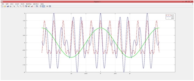
2-   A# In this example i will show you another 4 signals with another 4 responses with changing the frequencies and the phase angel.

So we will see 2 superposition signals and  1 fft and 1 cosine signal.

I defined it as shown in the figure using matlab file.

And in this example I used the function plot to show you the output.

Fig-4

                            Fig-5 FFT 

These applications can be used in time analysis of continuous systems or for describing a superposition in physics and electronics, or seeing the output of signal responses over the plot results. 

●  Matlab  Part2 in electricity and electronics for using this article:

Deblurring Images Using a Regularized Filter

Here we introduce a type of image filters using in diffrent domain and field.

This example shows how to use regularized deconvolution to deblur images.

Regularized deconvolution can be used effectively when constraints are applied on the recovered image 

(e.g., smoothness, pixels records,...) and

 Limited information is known about the additive noise.

 The blurred (!) and noisy image(!!) is restored by a constrained least square restoration algorithm(!!!) that uses a regularized filter.

Step 1: Read Image

The example reads in an RGB image and cropsit to be 256-by-256-by-3.

The deconvreg function can handle arrays of any dimension.

I = imread('tissue.png');

I = I(125+(1:256),1:256,:);

f1 = figure;

imshow(I);

figure(f1);

title('Original Image');

text(size(I,2),size(I,1)+15, ...

'Image courtesy of Alan Partin, Johns Hopkins University', ...

'FontSize',7,'HorizontalAlignment','right');

Step 2: Simulate a Blur and Noise

Simulate a real-life image that could be blurred (e.g., due to camera motion or lack of focus, or weak resolution,...) and noisy (e.g., due to randomdisturbances).

The example simulates the blur by convolving a Gaussian filter with the true image (using imfilter).

The Gaussian filter represents a point-spread function, PSF.

PSF = fspecial('gaussian',11,5);

Blurred = imfilter(I,PSF,'conv');

f2 = figure;

imshow(Blurred);

figure(f2);

title('Blurred');

We simulate the noise by adding a Gaussian noise of variance V to the blurred image (using imnoise).

V = .02;

BlurredNoisy = imnoise(Blurred,'gaussian',0,V);

f3 = figure;

imshow(BlurredNoisy);

figure(f3);

title('Blurred& Noisy');

Step 3: Restore the Blurred and Noisy Image

Restore the blurred and noisy image supplying noise power, NP, as the third input parameter.

To illustrate how sensitive the algorithm is to the value of noise power, NP, the example performs three restorations.

The first restoration, reg1, uses the true NP. Note that the example outputs two parameter shere.

 The first return value, reg1, is the restored image.

 The second return value, LAGRA, is a scalar, Lagrange multiplier, on which the deconvreg has converged.

This value is used later in the example.

NP = V*numel(I); % noise power

[reg1, LAGRA] = deconvreg(BlurredNoisy,PSF,NP);

f4 = figure;

imshow(reg1);

figure(f4);

title('Restoredwith NP');

The second restoration, reg2, uses a slightly over-estimated noise power, which leads to a poor resolution.

reg2 = deconvreg(BlurredNoisy,PSF,NP*1.3);

f5 = figure;

imshow(reg2);

figure(f5);

title('Restoredwithlarger NP');

The third restoration, reg3, is given an under-estimated NP value.

This leads to an overwhelming noise amplification and "ringing" from the image borders.

reg3 = deconvreg(BlurredNoisy,PSF,NP/1.3);

f6 = figure;

imshow(reg3);

figure(f6);

title('Restoredwithsmaller NP');

Step 4: Reduce Noise Amplification and Ringing

Reduce the noise amplification and "ringing" along the boundary of the image by calling the edge taper function prior to deconvolution.

Note how the image restorationbecomesless sensitive to the noise power parameter.

Use the noise power value NP from the previous example.

Edged = edgetaper(BlurredNoisy,PSF);

reg4 = deconvreg(Edged,PSF,NP/1.3);

f7 = figure;

imshow(reg4);

figure(f7);

title('Edgetapereffect');

Step 5: Use the Lagrange Multiplier

Restore the blurred and noisy image, assuming that the optimal solution is already found and the corresponding Lagrange multiplier, LAGRA, is given.

 In this case, any value passed for noise power, NP, is ignored.

To illustrate how sensitive the algorithm is to the LAGRA value, the example performs three restorations.

The first restoration (reg5) uses the LAGRA output from the earlier solution (LAGRA output from first solution in Step 3).

reg5 = deconvreg(Edged,PSF,[],LAGRA);

f8 = figure;

imshow(reg5);

figure(f8);

title('Restoredwith LAGRA');

The second restoration (reg6) uses 100*LAGRA which increases the significance of the constraint.

By default, this leads to over-smoothing of the image.

reg6 = deconvreg(Edged,PSF,[],LAGRA*100);

f9 = figure;

imshow(reg6);

figure(f9);

title('Restoredwith large LAGRA');

The third restoration uses LAGRA/100 which weakens the constraint (the smooth ness requirement set for the image).

It amplifies the noise and eventually leads to a pure inverse filtering for LAGRA = 0.

reg7 = deconvreg(Edged,PSF,[],LAGRA/100);

f10 = figure;

imshow(reg7);

figure(f10);

title('Restoredwithsmall LAGRA');

Step 6: Use a DifferentConstraint

Restore the blurred and noisy image using a different constraint (REGOP) in the search for the optimal solution.

 Instead of constraining the image smoothness (REGOP is Laplacian by default), constrain the image smoothness only in one dimension (1-D Laplacian).

REGOP = [1 -2 1];

reg8 = deconvreg(BlurredNoisy,PSF,[],LAGRA,REGOP);

f11 = figure;

imshow(reg8);

figure(f11);

title('Constrained by 1D Laplacian');