Matlab Simulink Modeling and architecture level 7.3

 

Level-24-3.1: in Matlab-simulink

24-3.2: in Automotive Matlab-simulink

24-3.3: in complex technologies and practices use :

Developpement in Matlab Simulink leveling from 2016;

Also designing leveling concepts for engineering;

Advanced leveling automatic control systems,

Specially in the vehicule fields, automotic control systems, in automotive systems and concepts, Epowertrain, modeling , etc. ,.

A+++Modeling an Automatic Transmission Controller

Fig-1

B+Here we will make a model of an automatic controller Fig-1:

a-Vehicle

b-Transmission

c-Shift logical control module part

d-Engine RPM part module component and parts

e-Manœuvres GUI part

f-Plot results of 3 output controlledsignals (Throttle(qi), Engine RPM(Vi), and Vehicle Speed(Qxi))

g-Complete controlled system of automatictransmitted in/out signals vehicle modules (parts, VTD,...).

                                                   Fig-2

                       

Fig-3

C+Modeling an Automatic Transmission Controller

Open Example

*This example shows how to model an automotivedrivetrainwith Simulink®.

**Stateflow® enhances the Simulink model with its representation of the transmission control logic concepts (forming nodal parts, concepts of IO, Concepts of UP/Down streams,...)-A and control modules (control nodal engineering, control of blackbody spots,...)-AA and units applications(+++)A+3.

***Simulink provides a powerful environment for the modeling and simulation of dynamic systems(cars(40% today) – trains(20 to 30%) and planes(8%)) and processes(+++4).

*In many systems, though, supervisory functions like changing modes or invoking new gain schedules (gainQSC) must respond to events that may occur and conditions that develop over time.

**In many systems we can add losses(LossesQSC), parasitics, critical pathes and critical topologies of control in each system depending on nomber of parameters and testing

experiences.

***As a result, the environment requires a language capable of managing these multiple modes and developing conditions.

*In the following example, Stateflow shows its strength in this capacity by performing the function of gear selection(QSCI) in an automatic transmission.

**This function is combined with the drive traind ynamics in a natural and intuitive manner by incorporating a Stateflow block in the Simulink block diagram[tool boxes modeling and standards ASPICE.4.03].

D+Maneuvers GUI part Fig-2, Fig-3, Fig-4, Fig-5

a- Variation in manevres between 4 cases passing manevre, gradual acceleration, hard breaking and

coasting.

b-Each had a limit charcheteristics concerning throttle(iiV), speed(iiVi) and breaking.

E+ Cylendeur cars and auto.

F+ Engine part modeling systems (Koncepten und methoden die autos hybride-elektisch) consisting of:

1-Torque parameters

2-Throttle component

3-Engine tourque 2 dimension graph, nowyoucanchangedin 3 dimension modelinggraphicalparameters and fonctions.

4-Amplifier

5-Integration part

6-Feedback coefficients

7-Diffrentiator

Matlab Simulink Developpement and Engineering

matlab

 Blog Developped from 2018 by Mr.Micheal ARMANIOUS.

Matlab Level 12.3 For Engineers in 

=>Planes, 

=>>Automobile, 

===>>> trains Applications;

Matlab-Simulink
----------------------------

Introduction :

Matlab Simulink use in many fields in signals analysis,

Systems, transfere functions, Digital systems, Planes,

Digital cameras and sensors and soon….

Firstly : I show you some Matlab Simulink Boxes :

1-A

Fig-1

Here there are many libraries consist each of them of many boxes 

Fig-2

and electrical electronics components and devices.

Example : HDL Coder ;

Can transfer all the components and the system architecture with 

it’s simulations in HDL Files, …

Another example continuous libraries you will find DC Sources, AC 

sources, continuous source signals and so on.

So  finally each library consists of 

electrical-electronic components and devices 

for electrical applications and architecture since all 

engineering fields as trains control circuits, cars signal analysis, 

planes and calculators architectures and so on……

Fig-3

°°°°°°°°°°°°°°°°°°°°°°°°°°°°°°°°°°°°°°°°°°°°°°°°°°°°°°°°°°°°°°°°°°°°°°°°°°°°°°°°°°°°°°°°°°°°°°°°

2- Applications in Matlab :

Methods and manipulations of image recognitions, image detection,...

Applications For image processing in the fields of medicine or research or spatial or electronics architectures and sensors developpements……. specailly in image processing.

Registering an Image Using Normalized Cross-Correlation

This example shows how to find a template image within a larger image.

Sometimes one image is a subset of another. Normalized cross-correlation can be used to determine how to register or align, or modifing the images by translating, 

translation methods one of them.

We here show how to read an image file , file name type png,….

Step 1: Read Image

onion = imread('onion.png');

peppers = imread('peppers.png');

imshow(onion)

figure, imshow(peppers)

Fig-4

Step 2: Choose Subregions of Each Image

It is important to choose regions that are similar.

The image sub_onion will be the template, and must be smaller than the image sub_peppers. You can get these sub regions using either the non-interactive script below or the interactive script.

You can use here the methods non-interactive or the other method interactive.

Firstly

% non-interactively

rect_onion = [111 33 65 58];

rect_peppers = [163 47 143 151];

sub_onion = imcrop(onion,rect_onion);

sub_peppers = imcrop(peppers,rect_peppers);

% OR

%Secondly             

% interactively

%[sub_onion,rect_onion] = imcrop(onion); % choose the pepper below the onion

%[sub_peppers,rect_peppers] = imcrop(peppers); % choose the whole onion

% display sub images

figure, imshow(sub_onion)

Fig-5

figure, imshow(sub_peppers)

Fig-7

°°°°°°°°°°°°°°°°°°°°°°°°°°°°°°°°°°°°°°°°°°°°°°°°°°°°°°°°°°°°°°°°°°°°°

3- Applications in Matlab :

Applications For Modeling Motor engines in Trains-Automobiles - Planes……. specailly used in timing, delays for engines in closed loop systems as Boost systems, Hydrolic systems, Oil closed loops with motor Engines and so on…………………..

Fig-8

 Engine Timing Model With  Closed Loop control

Conssisting of :

                       1-Contrôler- Controler, Calculator,..... (ECU, ECU2, ECM, UBM,….,…)

                       2- Speed Setting and settling Point

                       3- Throttle And Manifold

                       4- Compression

                       5- Combustion

                       6- Valve (new valves, new solinoids, new mechanisms) Timing and Delay

                       7- Engine Dynamics (transmission, other motros on the weels,...etc.)

                       8- Crank Speed

                       9-Scope to show Speed and Closed Loop outputs

                       10-Automatic EE, HYB, HEV,...etc

                                                                               Fig-9 Engine Speed

                                                      Fig-10 Engine Speed, Control axes

°°°°°°°°°°°°°°°°°°°°°°°°°°°°°°°°°°°°°°°°°°°°°°°°°°°°°°°°°°°°°°°°°°°°°°°°°°°°°°°°°°°°°°°°°°°°°°°°°°°°°°°°°°°°°°°°°°°°°°°°°°°°°°°°°

4- Electrical / electronics Signals :

I will show you my friends some examples using matlab in signal analysis and responses.

1-    a+ Firstly you know that:

Here using cosine signals in our application (Fig-1), but also if you want to calculate using sine signals you can write the fonctions as this.

I(t) = I_m cos (w*t)

I(t) = I_m cos ((2*pi*f )*t)

V(t) = V_m cos (w*t)

V(t) = V_m cos ((2*pi*f )*t)

………………………………………..

I(t) = I_m sin (w*t)

I(t) = I_m sin ((2*pi*f )*t)

V(t) = V_m sin (w*t)

V(t) = V_m sin ((2*pi*f )*t)

1-    b+ Secondly appling this equations in our example using matlab:

Now in this example i used and explaned the time domain inbetween –pi until +pi

so

I defined x between –pi until +pi.

Defined y1 using the addition or the superpossition of 2 cosine signals.

Y2 is the fast forrier transform of y1 in the time domain.

Y3 sa,ple cosine signal.

Also in y1 first signal is 2*pi*f + another signal of cosine type using amplitude of

0.5 v,  doubling the same cosine with the same phase (theta ø).

X remember is varies between –pi until + pi.

                                    Fig-11

Another thing figure(1) our figure will appear in this window output.

In the function subplot I used to define first part in the graph with colors to differentiate between function responses so y1 ---> red,  y2 ---> blue,  y3 ---> green.

                                               Fig-12

I show you the electrical functions in graph fig1,fig2, fig3 which using adding or superposition of  2 cosine functions, also fast furrier transform (fft),  a simple cosine signal.

                                          Fig-13

++++++++++++++++

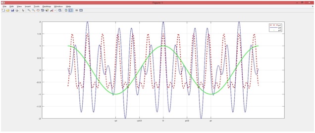
1-    In this example i will show you another 4 signals with another 4 responses with changing the frequencies and the phase angel.

So we will see 2 superposition signals and  1 fft and 1 cosine signal.

I defined it as shown in the figure using matlab file.

And in this example I used the function plot to show you the output.

Fig-14

                                                                   Fig-15

These applications can be used in time analysis of continuous systems or for describing a superposition in physics and electronics, or seeing the output of signal responses over the entire time domain interval.

+++++++++++++++++++++++++++++++++++++++++++++++++++++++++++++++++++++++++++++++++++++++++

Matlab  Part2 in electricity and electronics:

Matlab  Part2 in Image Sensors, Image Recognition, and Image

detection:

5- Image Sensors Architecture :

Deblurring Images Using a Regularized Filter

This example shows how to use regularized deconvolution to deblur images.

Regularized deconvolution can be used effectively when constraints are applied on the recovered image

 (e.g., smoothness, distortion, concentrated error detection,...) and limited information is known about the additive noise/or concentrated compound of noisy energy;....

The blurred and noisy image is restored by a constrained least square restoration algorithm that uses a regularized filter; you can defined also another algorithmic filters for the distortion parts; or compounds;....

Step 1: Read Image

onion = imread('onion.png');

peppers = imread('peppers.png');

imshow(onion)

figure, imshow(peppers)

                                                                     Fig-16

Fig-17

Step 2: Choose Subregions of Each Image

It is important to choose regions that are similar.

The image sub_onion will be the template, and must be smaller than the image sub_peppers. You can get these sub regions using either

:                                the non-interactive script below or the interactive script.

You can use here the methods non-interactive or the other method interactive.

Firstly

% non-interactively

rect_onion = [111 33 65 58];

rect_peppers = [163 47 143 151];

sub_onion = imcrop(onion,rect_onion);

sub_peppers = imcrop(peppers,rect_peppers);

% OR

%    Secondly             

% interactively

%[sub_onion,rect_onion] = imcrop(onion); % choose the pepper below the onion

%[sub_peppers,rect_peppers] = imcrop(peppers); % choose the whole onion

% display sub images/without the choosed part.

figure, imshow(sub_onion)

                          

Fig-18

figure, imshow(sub_peppers)

                            

                             

fig-19

Step 1: Read Image is related to the title in the previous part:

you will find it in Fig-6

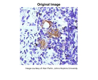
The example reads in an RGB image and cropsit to be 256-by-256-by-3.

The deconvreg function can handle arrays of any dimension.

I = imread('tissue.png');

I = I(125+(1:256),1:256,:);

f1 = figure;

imshow(I);

figure(f1);

title('Original Image');

text(size(I,2),size(I,1)+15, ...

'Image courtesy of Alan Partin, Johns Hopkins University', ...

'FontSize',7,'HorizontalAlignment','right');

Step 2: Simulate (by appling noisy) a Blur and Noise

step 2 here related to step 2 and 3 in the przvious part with there images fig- 7 and Fig 8;

Simulate a real-life image that could be blurred (e.g., due to camera motion or lack of focus) and noisy (e.g., due to random disturbances).

The example simulates the blur by convolving a Gaussian filter with the true image (usingimfilter).

The Gaussian filter represents a point-spread function, PSF.

PSF = fspecial('gaussian',11,5);

Blurred = imfilter(I,PSF,'conv');

f2 = figure;

imshow(Blurred);

figure(f2);

title('Blurred');

We simulate the noise by adding a Gaussian noise of variance V to the blurred image (using imnoise).

V = .02;

BlurredNoisy = imnoise(Blurred,'gaussian',0,V);

f3 = figure;

imshow(BlurredNoisy);

figure(f3);

title('Blurred& Noisy');

Step 3: Restore the Blurred and Noisy Image

Restore the blurred and noisy image supplying noise power, NP, as the third input parameter.

To illustrate how sensitive the algorithm is to the value of noise power, NP, the example performs three restorations.

The first restoration, reg1, uses the true NP. Note that the example outputs two parameter shere.

 The first return value, reg1, is the restored image.

 The second return value, LAGRA, is a scalar, Lagrange multiplier, on which the deconvreg has converged.

This value is used later in the example.

NP = V*numel(I); % noise power

[reg1, LAGRA] = deconvreg(BlurredNoisy,PSF,NP);

f4 = figure;

imshow(reg1);

figure(f4);

title('Restoredwith NP');

The second restoration, reg2, uses a slightly over-estimated noise power, which leads to a poor resolution.

reg2 = deconvreg(BlurredNoisy,PSF,NP*1.3);

f5 = figure;

imshow(reg2);

figure(f5);

title('Restoredwithlarger NP');

The third restoration, reg3, is given an under-estimated NP value.

This leads to an overwhelming noise amplification and "ringing" from the image borders.

reg3 = deconvreg(BlurredNoisy,PSF,NP/1.3);

f6 = figure;

imshow(reg3);

figure(f6);

title('Restoredwithsmaller NP');

                                        Fig-20

           

                              Fig-21

Step 4: Reduce Noise Amplification and Ringing

Reduce the noise amplification and "ringing" along the boundary of the image by calling the edge taper function prior to deconvolution.

Note how the image restorationbecomesless sensitive to the noise power parameter.

Use the noise power value NP from the previous example.

Edged = edgetaper(BlurredNoisy,PSF);

reg4 = deconvreg(Edged,PSF,NP/1.3);

f7 = figure;

imshow(reg4);

figure(f7);

title('Edgetapereffect');

Step 5: Use the Lagrange Multiplier

Restore the blurred and noisy image, assuming that the optimal solution is already found and the corresponding Lagrange multiplier, LAGRA, is given.

 In this case, any value passed for noise power, NP, is ignored.

To illustrate how sensitive the algorithm is to the LAGRA value, the example performs three restorations.

The first restoration (reg5) uses the LAGRA output from the earlier solution (LAGRA output from first solution in Step 3).

reg5 = deconvreg(Edged,PSF,[],LAGRA);

f8 = figure;

imshow(reg5);

figure(f8);

title('Restoredwith LAGRA');

The second restoration (reg6) uses 100*LAGRA which increases the significance of the constraint.

By default, this leads to over-smoothing of the image.

reg6 = deconvreg(Edged,PSF,[],LAGRA*100);

f9 = figure;

imshow(reg6);

figure(f9);

title('Restoredwith large LAGRA');

The third restoration uses LAGRA/100 which weakens the constraint (the smooth ness requirement set for the image).

It amplifies the noise and eventually leads to a pure inverse filtering for LAGRA = 0.

reg7 = deconvreg(Edged,PSF,[],LAGRA/100);

f10 = figure;

imshow(reg7);

figure(f10);

title('Restoredwithsmall LAGRA');

Step 6: Use a Different Constraint

Restore the blurred and noisy image using a different constraint (REGOP) in the search for the optimal solution.

 Instead of constraining the image smoothness (REGOP is Laplacian by default), constrain the image smoothness only in one dimension (1-D Laplacian).

REGOP = [1 -2 1];

reg8 = deconvreg(BlurredNoisy,PSF,[],LAGRA,REGOP);

f11 = figure;

imshow(reg8);

figure(f11);

title('Constrained by 1D Laplacian');

Another complete Image recognition and treatement;

Fig-22 Origin image, blurred image, noisy part, and treatment.

Conclusion:

A+++Matlab Level 12.3 For Engineers in 

=>Planes, 

=>>Automobile, 

===>>> trains Applications;

B+++Matlab Level 12.3 For Engineers in 

I show you some Matlab Simulink Boxes 

Applications in Matlab >>> 2:

 Applications in Matlab >>> 3- Planes Applications. :

4- Electrical / electronics Signals :

5- Image Sensors Architecture :

7- Restore the Blurred and Noisy Image: